NR 532 Project Sections
Instructor: Stacy Nelson
NR 532 is the second course in the core Geographic Information Systems (GIS) series and focuses on understanding the principle and theory of geographical sciences. The course content includes the fundamental spatial concepts that underpin every GIS as well as discussions of current Geographic Information Science issues.
The course covered the following topics:
- Basic GIS theory and principles, operations, and applications.
- The nature of geographic data.
- Concepts of uncertainty and error within geographic data.
- Concepts of spatial analysis.
- Ways to incorporate GIS techniques into your individual discipline of study.
Course Final Project
The objectives of the final project for NR 532 was to perform a geospatial analysis that brings together many of the concepts taught in the class and make a presentation addressing the the objectives, methadology, and results of the project.
Objectives
The United States, like any other large country, has a wide range of climates and environments. It has everything from torrid deserts to icy mountain peaks. The weather pattern in every part of the country is unique and determined by factors such as proximity to the ocean, geography, latitude and propensity for severe weather. Our assertion is that these weather phenomena have an effect on the cost of living in the US. In the analysis, we will use nationwide heating and cooling degree day averages along with wind gust frequencies to answer two basic questions:
- What is the relative cost of living in the US based on environmental factors such as heating and cooling costs?
- What is the relative cost of living with a factor for storm damage added?
Assumptions
- Energy costs are uniform across the country
- Environmental factors such as severe weather, flooding, tectonic activity, etc… should be weighted well below temperature influences due to low frequency of occurrence
Mean Total Heating and Cooling Degree Days
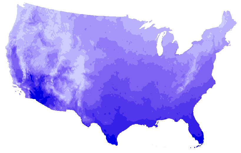
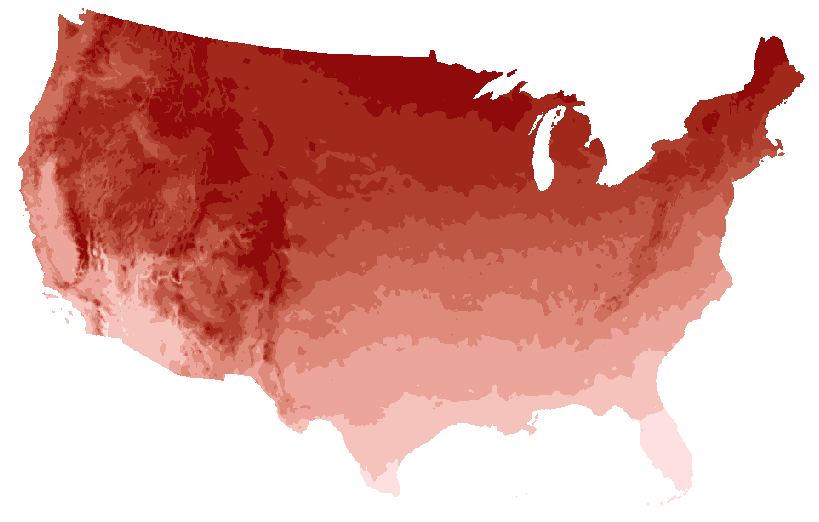
Mean Total Cooling Degree Days (left) and Mean Total Heating Degree Days (right). Click image to view larger version.
Degree Days are the most common and popular weather variable utilized for weather derivatives, energy trading, weather risk management and seasonal planning. Degree Days are a practical method for determining cumulative temperatures over the course of a season. Originally designed to evaluate energy demand and consumption, degree days are based on how far the average temperature departs from a human comfort level of 65 °F . Simply put, each degree of temperature above 65 °F is counted as one cooling degree day, and each degree of temperature below 65 °F is counted as one heating degree day. For example, a day with an average temperature of 80 °F will have 15 cooling degree days. The number of degree days accumulated in a day are proportional to the amount of heating/cooling you would have to do to a building to reach the human comfort level of 65 °F. The degree days are accumulated each day over the course of a heating/cooling season, and can be compared to a long term (multi-year) average, or normal, to see if that season was warmer or cooler than usual. The graphic to the right (click for larger version) shows normal heating degree day accumulations over the full heating season (Source: NESDIS, NOAA).
Mean Occurrences of Peak Gust > 50 mph
Mean Occurances of Peak Gust > 50 mph. Click image to view larger version.
This element was computed using data from the National Climatic Data Center's Summary of the Day First Order (TD-3210) database (NOAA, 2000a). The original data is in knots and was reported as the 5-second peak gust for the day. This element is given in whole days. For a given month, the mean monthly values were computed by taking the 30-year mean of the monthly count of days where the peak wind gust was at or above 50 miles per hour. Monthly counts of days with the identified peak gust were the sum of days where at least one peak gust observation exceeded the identified threshold. The mean annual value was computed by taking the 30-year mean of the yearly counts. The yearly counts were computed by summing their 12 monthly counts.
Data Source: http://lwf.ncdc.noaa.gov/oa/about/cdrom/climatls2/info/atlasad.html
In order to understand the combined importance of the given “Degree Days” models, spatial analysis of raster data was performed. To evaluate and interpret the geographic information, methods such as vector to raster conversion, raster reclassification and raster set addition were used. A flow chart on the next slide shows how input vector based files were converted to raster and reclassified. Two different raster calculations were then performed. One calculated the cost with wind not taken into account: [hdd_reclass] + [cdd_reclass]. The second one took all three factors, including wind, into account: [hdd_reclass] + [cdd_reclass] + [wind_reclass].
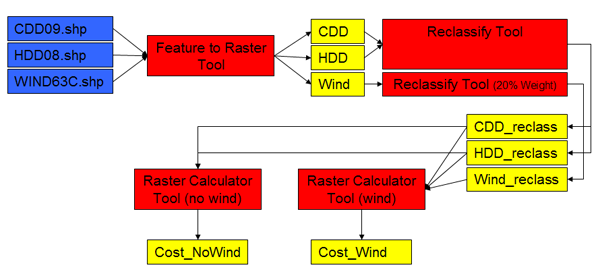
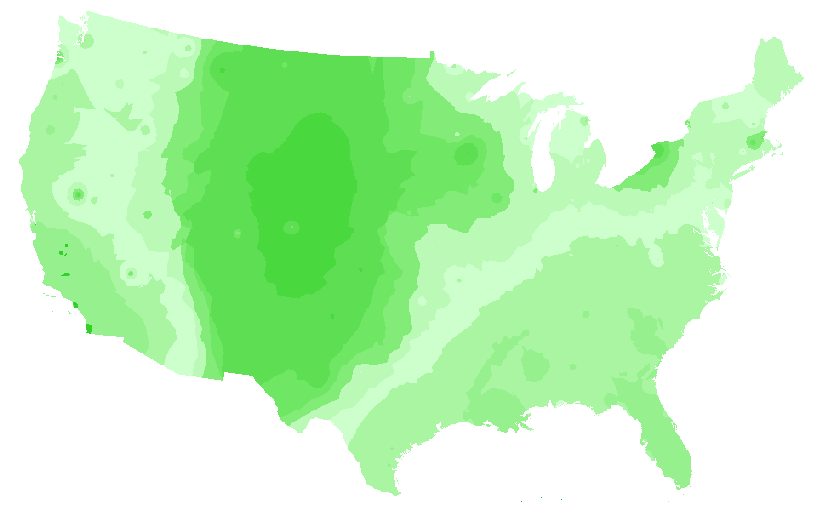
Project Methodology Flowchart
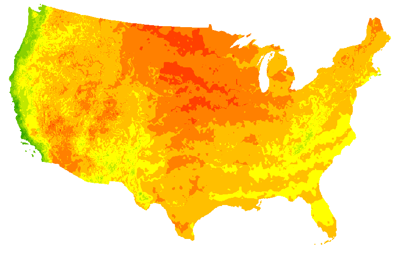
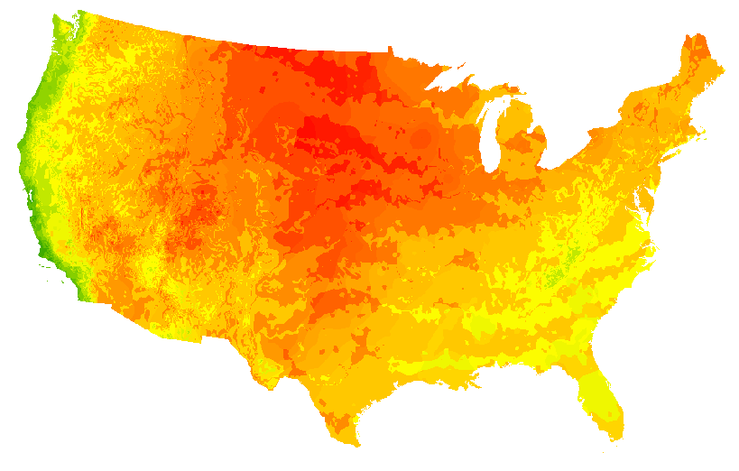
Relative cost of living based on heating and cooling only (left) and based on heating, cooling, and wind (right). Green equal lower cost of living and red equal higher cost of living. Click on the images for larger versions
Raster calculation results show that in general, environmental factors make the cost of living most expensive in the Midwestern states and least expensive on the immediate Pacific coast. The affect of storm damage from wind appears to have the greatest impact on the north-Midwestern states in the leeward area of the Rocky Mountains. The results appear to make sense. The influence of the Pacific Ocean limits extremes in temperatures along the coast. This means that people’s cost for heating and cooling is less then that of other part of countries. The East coast is different from the Pacific coast because the Gulf Stream acts as a catalyst for large weather systems, creating a wider gap between the average heating days and cooling days. This is especially evident in the Northeast where lake effect storms and east cost cyclogensis play large roles in the winter weather season. The results for Midwestern states are also logical. Stable temperatures are usually attributed to proximity of a geographic area to water. Because the Midwestern area is far from either ocean, they have the biggest temperature fluctuations and therefore a higher costs for heating and cooling. Results stemming from the analysis that included the wind factor are also not surprising. As stated above, the wind factor seems to have the biggest affect on the Midwestern states. This is not surprising because that area is leeward of the Rocky Mountains and is prone to frequent wind storms.