While ESRI's software is a valuable tool for many research applications, knowing the principles behind geospatial analysis independent of any specific software application is important. If you can apply the principles of geospatial analysis to a problem outside of any single software package, you have the ability to create a custom tool or set of tools to meet your research goals.
My research involves using and analyzing data from satellites the measure precipitation with active precipitation radar and passive microwave radiometers. The dataset generated by these satellites does not readily import into any common GIS application. As a result, I have to design custom tools and scripts for scientific data analysis tools like Matlab to perform any processing or analysis of the satellite data.
The following examples illustrate cases where geospatial analysis principles were used to design custom tools in order to investigate satellite derived data outside a typical GIS software environment.
Plotting the spatial and temporal distribution of a subset of precipitation features
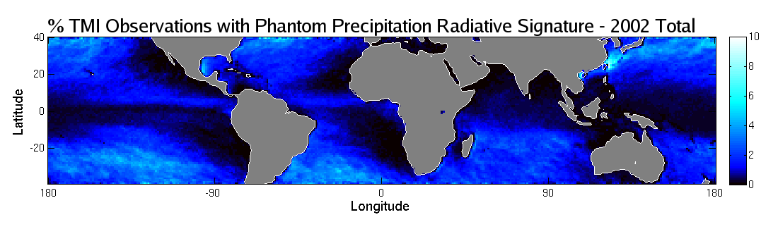
The total percentage of TMI observations with a phantom precipitation signature for 2002.
Click the image to view at full-size.
The above figure is a plot of a subset of precipitation - dubbed phantom precipitation - observed by NASA's Tropical Rainfall Measuring Mission (TRMM) satellite. The data in question is taken from the TRMM microwave radiometer (TMI). This raster dataset cover the TRMM observational domain and show the spatial extent of the feature of interest. The color coding of the individual pixels provides information about the temporal distribution (frequency of occurrence) of the feature of interest. The phantom precipitation was isolated from the dataset by filtering out data points that did not meet set of multi-spectral values and rain rate thresholds. The data analysis and plotting were done in Matlab.
Plotting Areas of Interest Based on Data from Multiple Sources
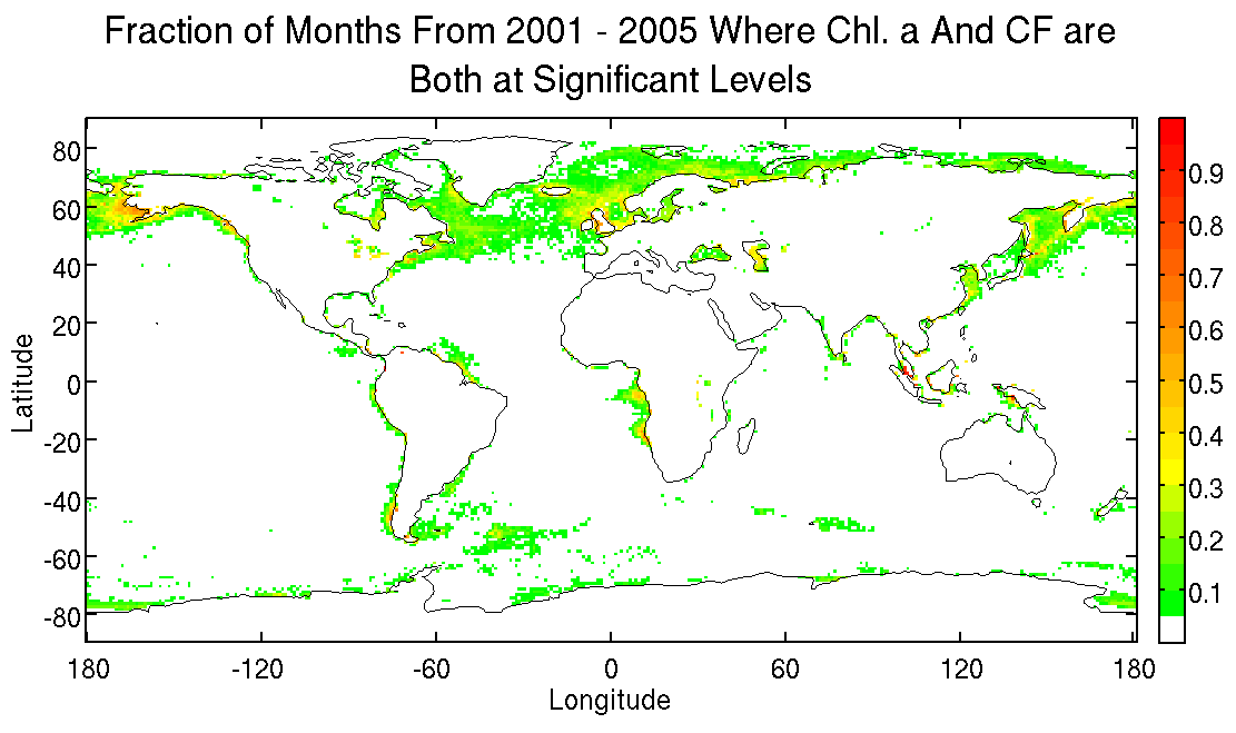
The fraction of month from 2001 - 2005 where chlorophyll a concentration is above 1.0 mg/m3 and MODIS derived cloud fraction is above 0.7.
Click the image to view at full-size.
The above figure shows the fraction of months with the in period from 2001 - 2005 where the SeaWiFFs estimated chlorophyll a concentration and the MODIS estimated cloud fraction are both above their given thresholds. The creation of this figure involved writing custom scripts to process the data from two different satellite instruments to a common spatial and temporal scale which could then be filtered for point matching the given criteria. The data analysis and plotting were done in Matlab.
Comparing Observations from Different Instruments
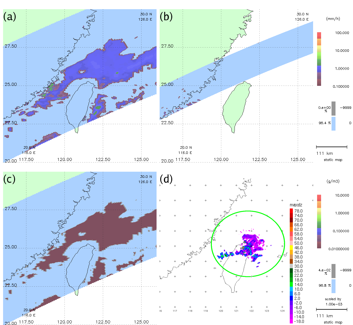
Phantom precipitation off the Taiwan coast on 1 Feb. 2000. (a) TMI surface precipitation retrieval. (b) PR near surface precipitation. (c) 14 km TMI cloud ice above observed cloud top level. (d) Coastal S-band radar composite. Ring denotes maximum range.
Click the image to view at full-size.
The above figure compares data from the TRMM TMI and precipitation radar as well as a WSR-88D S-band radar for an event off the northern coast of Taiwan. The challenge in creating this figure is in processing data of very different formats into a common projection and format so that the data collect from the different instrument can be examined for common features and differences. The data processing and analysis was done with a combination of NASA's TRMM orbit viewer and Zebra, a customized netCDF viewing and analysis application.